Deconstruction Series #1: Rebuilding GPT-2 in Pure C
Welcome to the GPT-2 Deconstruction Series — a deep dive into how GPT-2 really works, built from the ground up in pure C. No Python. No PyTorch. No magic. Just raw logic, memory management, and the beauty (and pain) of doing everything yourself.
Whether you’re here to learn how transformers tick, or just enjoy bending C to your will, this is your guide to building GPT-2 step by step — from tokenization to text generation.
Check Out the GPT-2 C Implementation: gpt2.c
In Part 1, we’ll lay the groundwork for running GPT-2 inference entirely in pure C. This includes:
- Understanding the GPT-2 architecture
- Extracting and loading model weights
- Building the Transformer block in C
- Tokenizing input and generating predictions manually
🚨 This is a learning-oriented reimplementation. It’s not meant to compete with optimized libraries like
ggml,transformers, orllama.cpp. The goal is understanding.
Architecture Summary: What is GPT-2?
GPT-2 is a stack of clever math layers that turns a sequence of words into predictions — one token at a time. Let’s walk through the key components in simple terms.
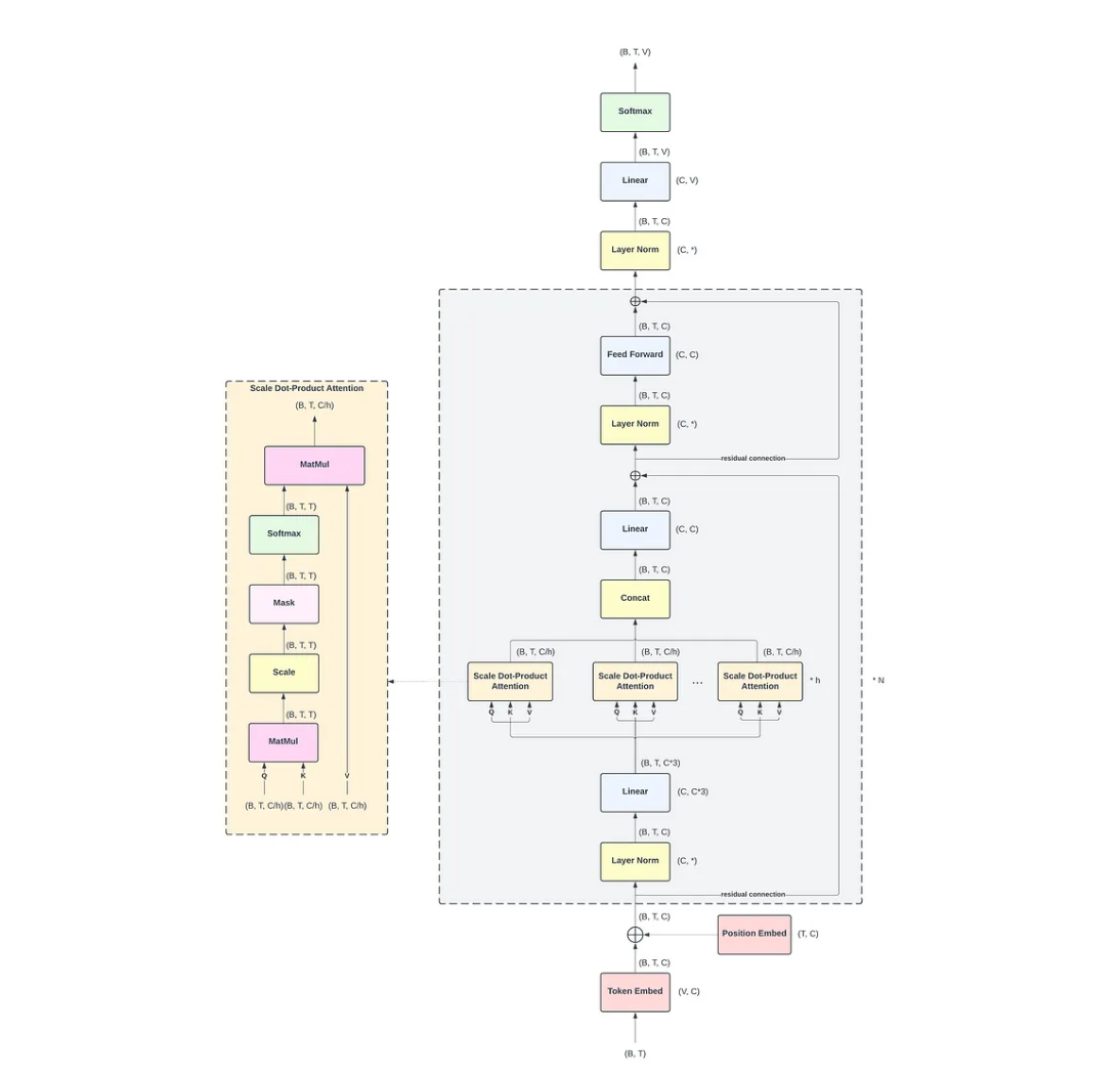
Token + Position Embeddings
“Give meaning to numbers.”
Before GPT-2 can process words, it needs to turn them into numbers. Each word or subword (called a token) is mapped to a high-dimensional vector using a token embedding.
-
The embedding table has size:
(vocab_size, hidden_size)
→ For GPT-2 small: (50257, 768)
That means each token becomes a 768-length float vector. -
The model also needs to know where each word appears in the sentence. So we add position embeddings — like saying “this is the 1st word, this is the 2nd,” etc.
Final input = token_embedding + position_embedding
N Transformer Blocks
“Stacked layers of thinking.”
GPT-2 uses 12 blocks (for GPT-2 Small). Each block contains two main sub-layers:
- Self-Attention
- MLP (Feedforward Network)
These layers are repeated again and again to refine the understanding of context.
Self-Attention (q, k, v, c_proj)
“Look at other words before making a decision.”
This is where GPT-2 pays attention to previous tokens to figure out what’s important. It breaks the input into three parts:
q= queriesk= keysv= values
Each is created by multiplying the input with a set of weights:
- Shapes:
q_weight,k_weight,v_weight: (hidden_size, hidden_size)
Full Attention Formula (Mathematical Form)
Inline math example: \(Q = XW^Q, \quad K = XW^K, \quad V = XW^V\)
Block math:
\[W^Q, W^K, W^V \in \mathbb{R}^{d_{\text{model}} \times d_{\text{head}}}\] \[d_{\text{head}} = \frac{d_{\text{model}}}{n_{\text{heads}}}\]Each GPT-2 attention block computes queries, keys, and values using linear projections from the input hidden state. These are then used for scaled dot-product attention.
Assuming:
n_embd = 768(hidden size)n_head = 12(number of attention heads)head_dim = n_embd / n_head = 64
Each token is transformed via three learned matrices: Q, K, and V.
| Projection | Weight Shape | Bias Shape | Description |
|---|---|---|---|
| Q (query) | (768, 768) | (768,) | Projects input to queries |
| K (key) | (768, 768) | (768,) | Projects input to keys |
| V (value) | (768, 768) | (768,) | Projects input to values |
| c_proj | (768, 768) | (768,) | Projects concatenated heads back to hidden |
MLP (Feedforward Network)
The MLP (Multi-Layer Perceptron) is the second major sub-layer in each GPT-2 transformer block. It operates independently on each token position after attention and helps the model learn deeper, nonlinear transformations.
The GPT-2 MLP is a simple two-layer fully connected network with a GELU activation in between:
Let:
n_embd= hidden size (e.g., 768 for GPT-2 small)n_inner= intermediate size (typically 4 ×n_embd= 3072)
Then the two layers have the following shapes:
| Layer | Weight Shape | Bias Shape |
|---|---|---|
| Linear₁ | (3072, 768) | (3072,) |
| Linear₂ | (768, 3072) | (768,) |
Note: PyTorch stores weights as (out_features, in_features)
Operations
- First linear layer (
c_fc) expands the hidden dimension:
h1 = x · W₁ᵗ + b₁ - GELU activation adds non-linearity:
h2 = GELU(h1) - Second linear layer (
c_proj) projects back to hidden size:
y = h2 · W₂ᵗ + b₂
Each operation is applied independently per token in the sequence.
Final Output: Vocabulary Projection and Sampling
After passing through all transformer layers, the final hidden state is projected back to the vocabulary space to generate the next token.
Vocabulary Projection
The final layer is a linear projection using the same weights as the token embedding:
\[\text{logits} = \text{hidden_state} \cdot W^\top\]Where:
hidden_statehas shape(seq_len, hidden_size)Wis the token embedding matrix of shape(vocab_size, hidden_size)- Result:
logitsshape is(seq_len, vocab_size)
Only the last token’s logits are used for next-token prediction.
Temperature Scaling
To control randomness, the logits are divided by a temperature value:
temperature = 1.0→ normal (unchanged) distribution< 1.0→ sharper, more confident choices (less randomness)> 1.0→ flatter distribution (more diversity)
🎲 Sampling
After temperature scaling, sampling determines which token to choose:
Greedy Sampling
- Select the token with the highest probability
- Deterministic, less creative
Top-k Sampling
- Keep only the
khighest-probability tokens - Sample randomly among them
Top-p (Nucleus) Sampling
- Keep the smallest set of tokens whose cumulative probability ≥
p - Sample from this dynamic shortlist
In C, you can implement sampling by:
- Applying softmax to logits
- Normalizing probabilities
- Picking based on random draw weighted by probabilities
Example
// Pseudocode
logits = matmul(last_hidden, embedding_T);
scaled_logits = logits / temperature;
next_token = sample_softmax_top_k(scaled_logits, k=40);